Python Machine Learning
Machine Learning (ML)
Types of Machine Learning algorithms
- Supervised
- Unsupervised
- Reinforcement Learning (RL)
- Semi-Supervised Learning (aka. Weak supervision) - uses some labeled data and some unlabeled data.
- Self-Supervised Learning (SSL) - self-supervised models generate implicit labels from unstructured data.
- Self-Supervised Learning
Supervised Learning
Models are trained on labeled data, where each input has a known correct output.
- We have a dataset with one or more “features” (or independent variables, or just variables) (X) and one or more results (y).
- We would like to create a function that given a new set of values for X will predict the value(s) of y.
It is called “supervised” learning because for the given data-set we know whay is the true result (aka. labels).
We can divide the supervised learning problems into two types:
-
Regression (continuous values)
-
Classification (discrete labels)
-
Input variables: Independent variables, aka. features
-
Output variables: Dependent variables, target, labels
The model is supposed to predict the output from the input.
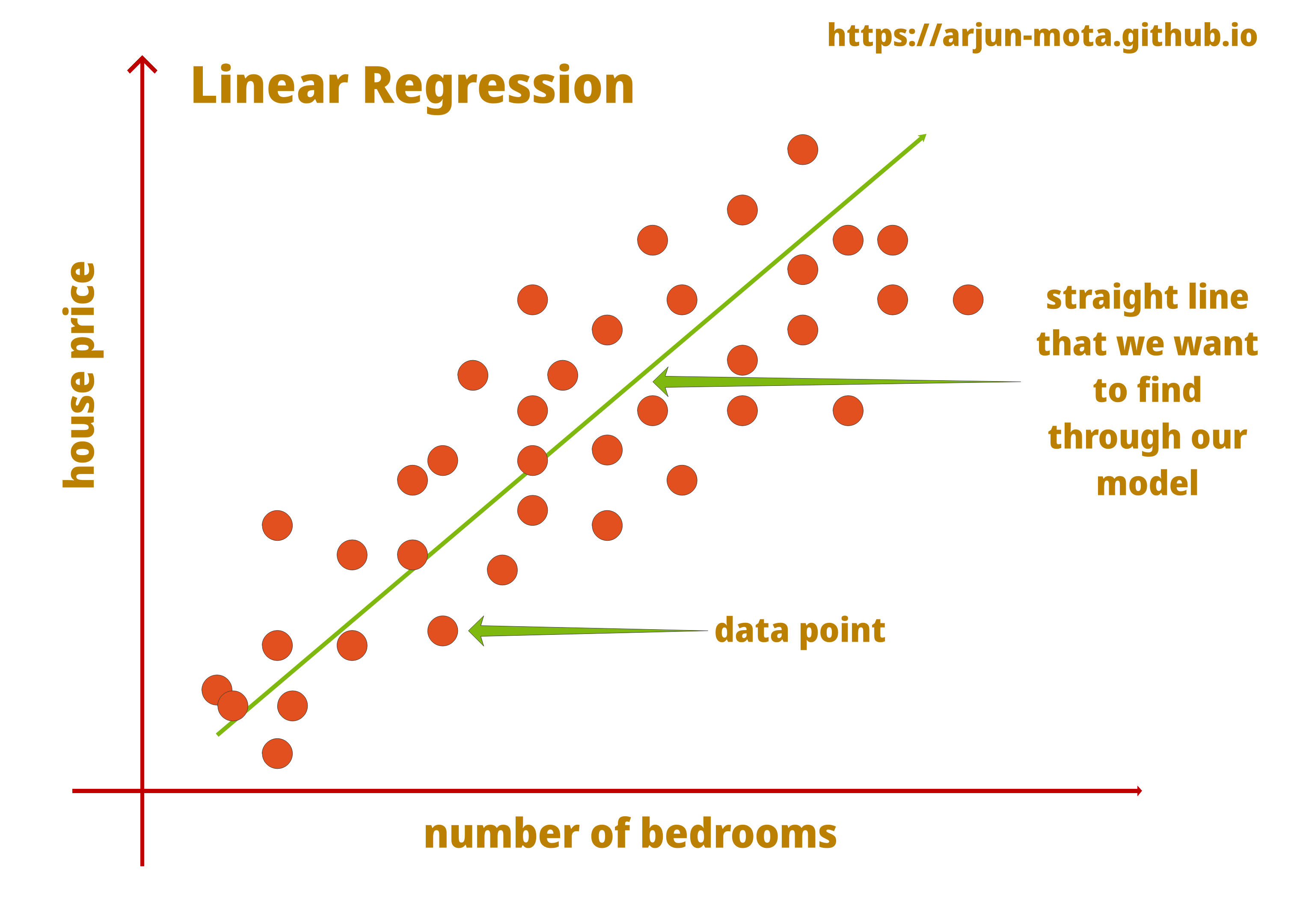
Regression problem
- Predict continuous valued output.

Housing prices (y)
-
X:
- Size of the flat in sqm.
- Distance from school.
- Distance from grocery store.
- City.
- Area in the city.
- …
-
How to predict the price based on the input variables?
Size, weight, color, nutrition value of various crops (y)
- X:
- rainfall
- amount of sun
- use of fertilizer
- …
Life expectancy at birth (y)
- X:
- alcohol or drug usage by the mother during the pregnancy
- age of the mother
- method of birth (delivery)
- birth-control used prior to the conception
- prior pregnencies
- same for the father where relevant
- A linear line:
ax + b? - Maybe a 2nd degree polynom
ax^2 + bx + c? - An exact match on the known points using very high degree polynom?
Classification problem
- Predict a discrete valued output (yes/no) or (A, B, C, D)
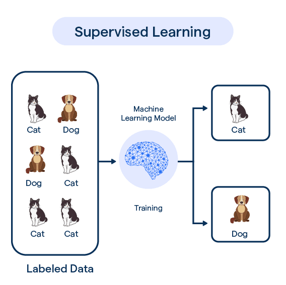
What kind of an animal is it? Is it a cat, a dog, a tiger?
X: * height * weight * size of ears, * size of tail * color, color of the eyes * … * OR the picture of an animal
Medical diagnosis
X: * Lab results * Images (CT, MRI, Ultrasound) * Patient metadata
- Brest Cancer: Tumor size (x). Is it malignant or benign (y)? Two distinct possibilities. Given a tumor (and its size) what is the probability that it is malignant?
- The Tumor size is a “feature”. In other problems we might have many more features.
- e.g. We might know the tumor size, the age of the patient, the gender of the patient, etc.
Iris species
- Classical example from the paper of Ronald Fisher in 1936: “The use of multiple measurements in taxonomic problems”
- y:
- Iris-setosa
- Iris-versicolor
- Iris-virginica
- X:
- sepal and petal length and width (4 numbers)
Unsupervised Learning
- Clustering (Divide by similarity)
Models are trained on unlabeled data and must discover structure on their own.
- We don’t have the right answer for the data set.
Customer Segmentation
- X:
- Purchase frequency
- Average order value
- Product categories
- Visit patterns
- y:
- Groups such as “high-value”, “occasional”, “price-sensitive”
Email categorization
-
X: Take a bunch of emails and create groups of messages. We can later name those groups (e.g. work, friends, family, marketing, spam, etc.)
-
News items
-
DNA sequences how much certains Genes are expressed
-
Social network analysis
-
Market segmentations
-
Astronomical data analysis
-
Cocktail party algorithm (separating two voices as recorded by two microphones) (Noise cancellation)
Clustering vs classification
Classification is when we have labeled data. It is a supervised method.
Clustering is when we don’t have labeled data and still would like to group (cluster) data-points according to their similarities. It is an unsupervised method.
Reinforcement Learning (RL)
- Mouse navigating in a maze.
- House cleaning robot.
- Waze?
Linear regression with sklearn
In this example we use some generated data to give a basic feeling.
In the first Jupiter Notebook file we see how we can train a model:
- examples/ml/basic_linear_regression.ipynb
Then we have two files, one using Jupyter notebook, one a plain Python file demonstrating how we can use the model.
- examples/ml/use_basic_linear_expression.ipynb
from joblib import load
import sys

if len(sys.argv) < 2:
    exit(f"Usage: {sys.argv[0]} Xes")

input_values = []
for val in sys.argv[1:]:
    input_values.append([float(val)])

model = load('linear.joblib')
print(model.predict(input_values))
examples/ml/basic_linear_regression.py
#get_ipython().system('pip install numpy pandas scikit-learn matplotlib joblib')

import sys
import numpy as np
import pandas as pd
from sklearn.linear_model import LinearRegression
import matplotlib.pyplot as plt
from joblib import dump
from sklearn.metrics import classification_report, confusion_matrix
from sklearn.model_selection import train_test_split

def generate_data_with_noise(size, noise_level):
    x = np.arange(size)
    noise = noise_level * (np.random.rand(size)-0.5)
    y = x + noise
    df = pd.DataFrame(data=[x, y]).T
    df = pd.DataFrame({"x":x, "y":y})
    return df

def main():
    if len(sys.argv) != 3:
        exit(f"Usage: {sys.argv[0]} SIZE NOISE")
    size, noise = int(sys.argv[1]), int(sys.argv[2])

    np.random.seed(42)
    df = generate_data_with_noise(size, noise)
    #df.plot()
    #df.plot.scatter(x='x', y='y', c='Blue');
    X = df[["x"]]
    #print(X)
    y = df["y"]
    print(y.head(3))

    #plt.scatter(X["x"], y, s=20);
    #plt.plot([0, size], [0, size], color="red");

    x_train, x_test, y_train, y_test = train_test_split(X, y, random_state=4)
    print(len(y_train), len(y_test))
    model = LinearRegression()
    model.fit(x_train, y_train)
    print(f"intercept: {model.intercept_}  coef: {model.coef_}")
    print('train coefficient of determination:', model.score(x_train, y_train))
    print('test coefficient of determination:', model.score(x_test, y_test))
    print('coefficient of determination:', model.score(X, y))

    x1, x2 = min(df["x"]), max(df["x"]) # 0, size-1
    y1, y2 = model.predict(pd.DataFrame({'x': [x1, x2]}))
    plt.plot([x1, x2], [y1, y2], color="red");
    plt.scatter(df["x"], df["y"]);
    plt.show()
    #dump(model, 'linear.joblib')

main()
Split data set to evaluate the model
- How can we really evaluate the model?
- We can check if using the model on the input data we trained it on will get predictions similar to what the real results were. If the error is too big then we know the model is not that good. If the predictions are very close to the real values then we might be happy. It is like testing students with the very same problems we have solved in the class-room. It gives you some level of confidence in the student, but how do you know if they can use that knowledge to solve other problems. How can you evaluate if they learned the material or only learned the answers to the specific questions you had in the class?
What we really would like to see is how the students (or our model) will fare with similar but not exactly same situation.
-
We need a new set of input data with the corresponding results.
-
Then using the model we can make predictions and we can compare the predictions to the actual data.
-
Instead of trying to get more data, what we usually do is take the original data-set and split it into two parts.
-
One part we’ll use to train the model and the other part we’ll use to test the model.
-
In supervised learning you receive a dataset of N elements (N rows) in each row you have X features (column) + 1 or more results y (also column)
-
You can divide the rows into two parts: training and testing.
-
You use the training part to train your model and you use the testing part to check how good your model can predict other values.
-
train_test_split()ofscikit-learncan do this. -
examples/ml/basic_linear_regression_more_data.ipynb
-
fix the seed by setting
random_stateto any fixed non-negative integer -
stratifysplitting for classification of inbalanced datasets
- train_test_split
Polynomial Regression
- When we allow for a function like
a + bx + cx^2 + dx^4 ...(given a single feature x)
polynomial_regression.ipynb
#get_ipython().system('pip install numpy pandas scikit-learn matplotlib joblib')

import sys
import numpy as np
import pandas as pd
from sklearn.linear_model import LinearRegression
from sklearn.preprocessing import PolynomialFeatures
from sklearn.pipeline import Pipeline
import matplotlib.pyplot as plt
from joblib import dump
from sklearn.metrics import classification_report, confusion_matrix
from sklearn.model_selection import train_test_split


def generate_data_with_noise(size, noise_level):
    x = np.arange(size)
    noise = noise_level * (np.random.rand(size)-0.5)
    y = x*x + noise
    df = pd.DataFrame(data=[x, y]).T
    df = pd.DataFrame({"x":x, "y":y})
    return df

def main():
    if len(sys.argv) != 4:
        exit(f"Usage: {sys.argv[0]} SIZE NOISE MODE")
    size, noise, mode = int(sys.argv[1]), int(sys.argv[2]), sys.argv[3]

    np.random.seed(42)
    df = generate_data_with_noise(size, noise)
    print(df)
    #df.plot()
    #df.plot.scatter(x='x', y='y', c='Blue');
    #plt.show()
    X = df[["x"]]
    #print(X)
    y = df["y"]
    print(y.head(3))

    x_train, x_test, y_train, y_test = train_test_split(X, y, random_state=4)
    print(len(y_train), len(y_test))

    if mode == "P":
        model = Pipeline([
            ('poly_features', PolynomialFeatures(degree=3)),
            ('linear_regression', LinearRegression())
        ])
    elif mode == "L":
        model = LinearRegression()
    else:
        exit(f"Invalid mode {mode}")


    model.fit(x_train, y_train)
    #print(f"intercept: {model.intercept_}  coef: {model.coef_}")
    print('train coefficient of determination:', model.score(x_train, y_train))
    print('test coefficient of determination:', model.score(x_test, y_test))

    #x1, x2 = min(df["x"]), max(df["x"]) # 0, size-1
    #y1, y2 = model.predict(pd.DataFrame({'x': [x1, x2]}))
    #plt.plot([x1, x2], [y1, y2], color="red");
    #plt.scatter(df["x"], df["y"]);
    #plt.show()
    #dump(model, 'linear.joblib')


main()
Food-truck linear regression
- examples/ml/food-truck.csv from the first exercise of the Machine learning course of Andrew Ng
- examples/ml/food-truck.ipynb
Basic Classification example
- examples/ml/basic_classification.ipynb
California Housing prices
from sklearn import datasets
from sklearn.model_selection import train_test_split
from sklearn.linear_model import LinearRegression
from sklearn.metrics import r2_score
from sklearn.preprocessing import PolynomialFeatures
from sklearn.ensemble import HistGradientBoostingRegressor, GradientBoostingRegressor, RandomForestRegressor
import time

def train_and_check(X, y):
    X_train, X_test, y_train, y_test = train_test_split(X, y, test_size=0.2, random_state=432)
    # random_state fixes the randomness

    model = LinearRegression()
    model.fit(X_train, y_train)
    prediction = model.predict(X_test)
    r2 = r2_score(y_test, prediction)
    print(f"r2: {r2}")

def train_and_check_with_model(model, X, y):
        start = time.time()
        X_train, X_test, y_train, y_test = train_test_split(X, y, test_size=0.2, random_state=432)
        model.fit(X_train, y_train)
        prediction = model.predict(X_test)
        r2 = r2_score(y_test, prediction)
        end = time.time()
        name = model.__class__.__name__
        print(f"{name:25} score: {r2} time: {end-start}")


def get_the_data_directly():
    housing = datasets.fetch_california_housing()
    #print(housing.__class__) # sklearn.utils._bunch.Bunch
    #print(housing.feature_names)
    X = housing.data
    y = housing.target

    print(X[0])
    print(y[0])

    return X, y

def get_the_data_as_a_pandas_data_frame():
    housing = datasets.fetch_california_housing(as_frame=True)
    #print(housing.__class__) # sklearn.utils._bunch.Bunch
    #print(housing.feature_names)
    df = housing.frame
    #print(df.__class__)  # pandas.core.frame.DataFrame
    #print(df.columns)

    y = df["MedHouseVal"]
    X = df.drop(columns=["MedHouseVal"])
    print(X.head(1))
    #print(X.iloc[0])
    print(y[0])

    return X, y

def main():
    X, y = get_the_data_directly()
    #X, y = get_the_data_as_a_pandas_data_frame()

    train_and_check(X, y)

    # Optimizations

    # poly = PolynomialFeatures()
    # print(X.shape)
    # X = poly.fit_transform(X)
    # print(X.shape)
    # train_and_check(X, y)

    # What are the extra features?
    # room size ->  (room size)^2
    # rooms * population

    # LR = LinearRegression()
    # GBR = GradientBoostingRegressor()
    # RFR = RandomForestRegressor()

    # for model in [LR, GBR, RFR]:
    #     train_and_check_with_model(model, X, y)

    # Improve and reduce time
    #HGBR = HistGradientBoostingRegressor()
    # use all the cores of the computer to reduce time
    #RFR_all = RandomForestRegressor(n_jobs=-1)

    # Hyperparameterization
    # for max_iter in [100, 150, 200, 250, 300]:
    #     model = HistGradientBoostingRegressor(
    #         max_iter=max_iter
    #     )
    #     print(f"max_iter: {max_iter}", end=" ")
    #     train_and_check_with_model(model, X, y)

    # for learning_rate in [0.2, 0.1, 0.05, 0.001]:
    #     for max_iter in [100, 150, 200, 250, 300]:
    #         model = HistGradientBoostingRegressor(
    #             max_iter=max_iter,
    #             learning_rate=learning_rate,
    #         )
    #         print(f"max_iter: {max_iter} learning_rate: {learning_rate}", end=" ")
    #         train_and_check_with_model(model, X, y)


main()
Kaggle
Kaggle - USA housing listing
- examples/ml/usa-housing-listings.ipynb
Kaggle - Iris
-
iris
-
examples/ml/iris.ipynb
Data Preprocessing
- Data Cleaning
- Removing duplicates
- Handling missing values
- Data Transformation
- Scaling
- Encoding
- Data integration (from multiple sources)
- Joining (combine rows from multiple tables based on an index)
- Merging (based on various columns)
- Data Reduction
- Sampling
- Dimensionality Reduction
Machine Learning 2
Number of features
- Can be large.
- Infinite number of features?
Linear regression
Housing prices (size in feet => price in USD)
-
m - number of examples in the dataset
-
X’s - input variables, features
-
y’s - output variables, target variables
-
(X, y) - single training example
-
(Xi, yi) - i-th training example
-
Training set => Learning Algorithm => h (hypothesis)
-
is function that converts X to estimated y.
y = h(X)as it is a linear function we can also write h(x) = ax^2 + b (a, b could be theta 0 and 1) -
Linear regression with one variable (aka.) Univariate Linear regression.
Cost function
-
Squared error function:
J(a, b) = (sum of (h(xi) - yi)^2)/2mwhereh(x) = ax^2 + b -
It is probably the most common used for linear regression problems because it seems to work the best in most cases.
-
We would like to find
aandbsoJ(a, b)is minimal. -
If we assume b=0 then we are looking at
min(J(a, 0))which is a 2D function -
In the general case though
min(J(a, b))is a 3D function for which we need to find the minimum -
Contour plots (contour figures)
Gradient descent
-
Gradient descent a generic algorithm to find a local minimum of a function.
-
Start at a random location.
-
Make a small step downhill.
-
Stop when around you everything is higher than where you are.
-
Problem is that depending on the starting point this can lead us to different local(!) minumum.
-
Learning rate (alpha) - the size of the steps we take on every iteration.
-
Derivative term - (a function of a and b).
-
If the learning rate is too large, the algorithm might diverge.
-
If the learning rate is too small, it might take a lot of steps to converge.
Gradient descent can converge even if the learning rate is fixed because the closer we get to the local minimum, the derivative of the cost function is smaller (closer to 0) and thus the multiplication of the cost function by the derivative is going to be smaller and the step we take is going to be smaller.
-
The above cost function of Linear regression is a Convex function so there is only one local minimum which is also the global minimum.
-
“Batch” Gradient Descent - means that at every step we use all the training examples.
-
There are other versions of Gradient descent.
Matrices
- Dimension of matrix = number of rows x number of columns (4x3)
- Addition of two matrices of the same dimension - element wise (same for subtraction)
- “Scalar Multiplication” - Multiplication of a matrix by a scalar (multiply each element by the scalar) (also scalar division)
R(3,2) x R(2) = R(3)multiply a matrix of 3 rows and 2 columns by a vector of 2 element (2 rows) (element-wise mnultiple and then sum the results)- 3x2 matrix multiply by a 2x1 matrix the result is 3x1 matrix
R(m, n) x R(n) = R(m)
| 1  3 |   | 1 |   | 16 |
| 4  0 | x | 5 | = |  4 |
| 2  1 |           |  7 |
- Matrix Matrix Multiplication
R(m,n) x R(n,k) = R(m, k)
| 1 3 2 |    | 1 3 |   | 11 10 |
| 4 0 1 | x  | 0 1 | = |  9 14 |
             | 5 2 |
-
Matrix multiplication is not commutative, that is
A x Bis not the same asB x A. -
Matrix multiplication is associative, that is
(A x B) x Cis the same asA x (B x C) -
Identity Matrix I or
I(nxn)is a square matrix in which everything is 0 except the diagonal that is filled with the number 1. -
A x I = I x A = A -
Matrix Inverse
A x A(to the power of -1) = I- Only square matrices have inverse, but not all square matrices have inverse. (e.g. the all 0s matrix does not have one) -
The matricses that don’t have an invers are somehow close to the all 0 matrix. They are also called “singular” or “degenerate” matrices.
-
Matrix Transpose - (1st row becomes the 1st column; 2nd row becomes 2nd column, etc….)
Machine Learning - Multiple features
-
n - number of features (number of columns in the table)
-
last column might be called y (the result)
-
m - number of samples (number of rows)
-
x(i) - row i, vector of values of a sample
-
x(i, j) - the value of row i column j
-
Also called “Multivariate linear regression”
-
Gradient descent for Multiple features
Feature Scaling
-
If one feature has numbers in the range of 0-2000 and the other feature has in the range of 0-5 then the inequality can make it much harder for the gradient descent to reach the minimum. It is better to have all the features in the same range of numbers. We can normalize the values by let’s say dividing each number by the max value of that feature. We might prefer that each feature will be in the range of
-1 <= value <= 1. This is not a hard rule though. -
Mean normalization - replace
xiwithx(i) - mu(i)where mu(i) is the mean or average of that feature. This way the feature will have 0 mean. Also:(x(i)-mu(i))/std(i)where mu(i) is the mean andstd(i)is the standard deviation.
Gradient Descent - Learning Rate
- Draw the graph of the value of the cost function as a function of the number of iterations in gradient descent.
- It should have a dowwards slope, but after a while its descent might slow down. (It is hard to tell how many iterations it will take.)
- If the convergence is some small (e.g. less than 1/1000 or epsylon, but it might be difficult to choose this number)
- If it is increasing than probably the learning rate is too big and it will never converge. (Fix is to use smaller learning rate.)
Features
- We can defined new features based on other features. (e.g. multiply two feature by each other to get the new feature)
Normal Equation
- An analytical way to find the best function
numpy.linalg.pinv(x.transpose * x) * x.transpose * y
-
Gradient Descent vs. Normal Equation
-
The latter migh work faster but only if the number of features is small. n = 10,000 might be the limit, depending on the computer power.
-
Noninvertibility
-
Redundant features: If two features are linearly dependent then the matrix is noninvertable (e.g. area in square mater and square feet)
-
Too many features (m <= n) - delete some features or use regularization
Multiple features
- Function of more than one X
exmaples/ml/multi_feature_linear_regression.ipynb
Logistic regression (for classification)
- Email: spam or not spam
- Tumor: malignant or benign
- Online Transaction: Fraudlent or not?
Binary classification:
y can be either 0 or 1,
- 0 = Negative class
- 1 = Positive class
Multi-class classification problem when y can have more than 2 distinct values
-
Linear regression using a threshold value
-
Decision boundary
-
The “Logistic regression cost function” based on the Sigmoid function is a non-convex function so Gradient Descent isn’t guarnteed to reach global minimum. So intead of that we use some log() function.
Optimization algorithms
- Gradient descent
- Conjugate gradient
- BFGS
- L-BFGS
The other 3 algorthms have the advantage of not needing to pick a alfa (learning pace), and they are often faster than Gradient descent. However they are more complex to implement.
Multi-feature Classification (Iris)
- iris
multi_feature_classification_iris.ipynb
Kaggle - Melbourne housing listing
- examples/ml/melbourne-housing-snapshot.ipynb
Machine Learning Resources
Regression Analyzis
Ways to measure correctness of a model
Classification Analysis
- Accuracy
- Precision
- Recall
- F1 Score
Unbiased evaluation of a model
- Assesment
- Validation
We need fresh data that has not been seen by the model before.
Splitting data
- Trainig set - for training, fitting the model, finding optimal coefficients.
- Validation set - for evaluation, hyperparameter tuning, performance assesment.
- Test set - unbiased evaluation of the model.
Also to notice:
- Underfitting
- Overfitting
Model selection and validation
- sckit-learn model_selection
- Cross validation (e.g. K-fold validation)
- Learning curves
- Hyperparameter tuning
K-fold valiadtion
-
divide the data into k (5-10) subsets
-
do the training and testing on each subset
-
each tim use one fold as the test-set and all the other folds as the train set
-
KFold()
-
StratifiedKFold()
-
LeaveOneOut()
Learning Curves
- The relation of data-set size in training and the score
- Find the optimal training size for best score in a reasonable time/dataset size.
Hypermatameter tuning (optimization)
- to determine the best model parameters
- GridSearchCV()
- RandomizedSearchCV()
- validation_curve()
The k-Nearest Neighbors (kNN)
import requests
import os
import shutil
import matplotlib.pyplot as plt
import pandas as pd
from sklearn.model_selection import train_test_split
from sklearn.neighbors import KNeighborsRegressor
from sklearn.metrics import mean_squared_error
from math import sqrt
import seaborn as sns
from sklearn.model_selection import GridSearchCV
from sklearn.ensemble import BaggingRegressor


def get_files():
    data_url =  "https://archive.ics.uci.edu/ml/machine-learning-databases/abalone/abalone.data"
    names_url = "https://archive.ics.uci.edu/ml/machine-learning-databases/abalone/abalone.names"

    filenames = []
    for url in (data_url, names_url):
        filename = url.split('/')[-1]
        filenames.append(filename)
        if not os.path.exists(filename):
            with requests.get(url, stream=True) as response:
                with open(filename, 'wb') as fh:
                    shutil.copyfileobj(response.raw, fh)
    return filenames


if __name__ == "__main__":
    data_file, names_file = get_files()
    columns = ["Sex", "Length", "Diameter", "Height", "Whole weight", "Shucked weight", "Viscera weight", "Shell weight", "Rings"]
    df = pd.read_csv(data_file, names=columns)
    #print(df.head())
    df = df.drop("Sex", axis=1)
    #print(df.head())

    #df["Rings"].hist(bins=15)
    #plt.show()

    #correlation_matrix = df.corr()
    #print(correlation_matrix["Rings"])

    X = df.drop("Rings", axis=1)
    X = X.values
    y = df["Rings"]
    y = y.values

    X_train, X_test, y_train, y_test = train_test_split(X, y, random_state=0)
    knn_model = KNeighborsRegressor(n_neighbors=3).fit(X_train, y_train)


    train_predictions = knn_model.predict(X_train)
    train_mse = mean_squared_error(y_train, train_predictions)
    train_rmse = sqrt(train_mse)
    print(train_rmse) # 1.67

    test_predictions = knn_model.predict(X_test)
    test_mse = mean_squared_error(y_test, test_predictions)
    test_rmse = sqrt(test_mse)
    print(test_rmse) # 2.36
    # That is the number of years as errors between the prediction and the actual value
    # This looks like overfitting

    # cmap = sns.cubehelix_palette(as_cmap=True)
    # f, ax = plt.subplots()
    # # Length and Diameter, the two columns with strong correllation
    # points = ax.scatter(X_test[:, 0], X_test[:, 1], c=test_predictions, s=50, cmap=cmap)
    # f.colorbar(points)
    # plt.show()

    # cmap = sns.cubehelix_palette(as_cmap=True)
    # f, ax = plt.subplots()
    # # Length and Diameter, the two columns with strong correllation
    # points = ax.scatter(X_test[:, 0], X_test[:, 1], c=y_test, s=50, cmap=cmap)
    # f.colorbar(points)
    # plt.show()


    # Tuning Hypermarameters
    # What should be the value of k ? k = 1 means you depend too much on a potentially outlier neighbour
    # If k is all the neighbours then for every prediction you will get the same answer.

    # Look for the best value for k in the range of 1-50
    # parameters = {"n_neighbors": range(1, 50)}
    # gridsearch = GridSearchCV(KNeighborsRegressor(), parameters)
    # gscv = gridsearch.fit(X_train, y_train)
    # # print(gscv)
    # print(gridsearch.best_params_)  # {'n_neighbors': 17}

    # train_preds_grid = gridsearch.predict(X_train)
    # train_mse = mean_squared_error(y_train, train_preds_grid)
    # train_rmse = sqrt(train_mse)
    # test_preds_grid = gridsearch.predict(X_test)
    # test_mse = mean_squared_error(y_test, test_preds_grid)
    # test_rmse = sqrt(test_mse)
    # print(train_rmse)
    # print(test_rmse)


    # Weighted Average of Neighbors Based on Distance

    parameters = {
        "n_neighbors": range(1, 50),
        "weights": ["uniform", "distance"],
    }
    gridsearch = GridSearchCV(KNeighborsRegressor(), parameters)
    gridsearch.fit(X_train, y_train)
    # print(gridsearch.best_params_)  # {'n_neighbors': 17}
    # train_preds_grid = gridsearch.predict(X_train)
    # train_mse = mean_squared_error(y_train, train_preds_grid)
    # train_rmse = sqrt(train_mse)
    # test_preds_grid = gridsearch.predict(X_test)
    # test_mse = mean_squared_error(y_test, test_preds_grid)
    # test_rmse = sqrt(test_mse)
    # print(train_rmse)
    # print(test_rmse)

    best_k = gridsearch.best_params_["n_neighbors"]
    best_weights = gridsearch.best_params_["weights"]
    bagged_knn = KNeighborsRegressor(
        n_neighbors=best_k, weights=best_weights
    )

    bagging_model = BaggingRegressor(bagged_knn, n_estimators=100)
    bagging_model.fit(X_train, y_train)
    train_preds_grid = bagging_model.predict(X_train)
    train_mse = mean_squared_error(y_train, train_preds_grid)
    train_rmse = sqrt(train_mse)
    test_preds_grid = bagging_model.predict(X_test)
    test_mse = mean_squared_error(y_test, test_preds_grid)
    test_rmse = sqrt(test_mse)
    print(train_rmse)
    print(test_rmse)
K-Means Clustering
Boston housing prices
from sklearn.datasets import load_boston
from sklearn.model_selection import train_test_split
from sklearn.linear_model import LinearRegression
from sklearn.ensemble import GradientBoostingRegressor
from sklearn.ensemble import RandomForestRegressor

x, y = load_boston(return_X_y=True)
print(x.shape)
print(y.shape)
#print(x)
#print(y)


x_train, x_test, y_train, y_test = train_test_split(x, y, test_size=0.4, random_state=0)

linear_model = LinearRegression().fit(x_train, y_train)
print(f"LinearRegression score train: {linear_model.score(x_train, y_train)}")
print(f"LinearRegression score test: {linear_model.score(x_test, y_test)}")

gradient_model = GradientBoostingRegressor(random_state=0).fit(x_train, y_train)
print(f"GradientBoostingRegressor score train: {gradient_model.score(x_train, y_train)}")
print(f"GradientBoostingRegressor score test: {gradient_model.score(x_test, y_test)}")

forest_model = RandomForestRegressor(random_state=0).fit(x_train, y_train)
print(f"RandomForestRegressor score train: {forest_model.score(x_train, y_train)}")
print(f"RandomForestRegressor score test: {forest_model.score(x_test, y_test)}")
Decision Tree
- Measure the the Mean Absolute Error of both the training and testing set
from sklearn.metrics import mean_absolute_error - too shallow: underfitting
- too deep: overfitting
Random Forrest
remove outlier from food-track calculate smallest profitable city
Resnet 50
import os
import sys
import cv2
import numpy as np
from tensorflow.keras.applications.resnet50 import ResNet50

if len(sys.argv) < 2:
    exit(f"{sys.argv[0]} IMAGEs")


os.environ['TF_CPP_MIN_LOG_LEVEL'] = '2'

# https://github.com/fchollet/deep-learning-models/releases/download/v0.2/resnet50_weights_tf_dim_ordering_tf_kernels_notop.h5
resnet50_weights = 'resnet50_weights_tf_dim_ordering_tf_kernels_notop.h5'
#rn50 = ResNet50(include_top=False, weights=None, pooling='avg')
#rn50 = ResNet50(include_top=False, weights=resnet50_weights, pooling='avg', input_shape=(512, 128, 1)) #(256, 256, 3))
rn50 = ResNet50(weights=resnet50_weights) #(256, 256, 3))
#rn50 = ResNet50(include_top=False, weights=None, input_shape=(640, 480, 3), pooling='avg')
#rn50 = ResNet50(include_top=False, weights=None)
#rn50 = ResNet50(include_top=False, weights="imagenet", pooling="avg")


#rn50.load_weights(resnet50_weights)
exit()
target_size = (640, 480)

for path in sys.argv[1:]:
    print(path)
    im = cv2.imread(path)
    print(im.shape)
    im = cv2.resize(im, target_size)
    print(im.shape)
    #old = im.copy()
    #im[0][0][0] = 0
    #im = cv2.cvtColor(im, cv2.COLOR_BGR2RGB) / 255.
    #print(np.array_equal(old, im))
    im = im[np.newaxis, ...]
    act = rn50.predict(im)
    print(act)